How to Make a Compound Interest Calculator in Microsoft Excel
Make your own versatile compound interest calculator in Microsoft Excel spreadsheet with the help of this article.
Compound interest calculators are easy enough to find online for free but they’re not as detailed and transparent as you’ll sometimes want them to be. You may be wanting to dissect the details of your compound calculation, wanting to project an investment’s performance or just gauge where your savings account will be sitting in a few years time. With this method you’ll be able to see not only the years but months, days or any time interval you see fit for your compounded interest returns.
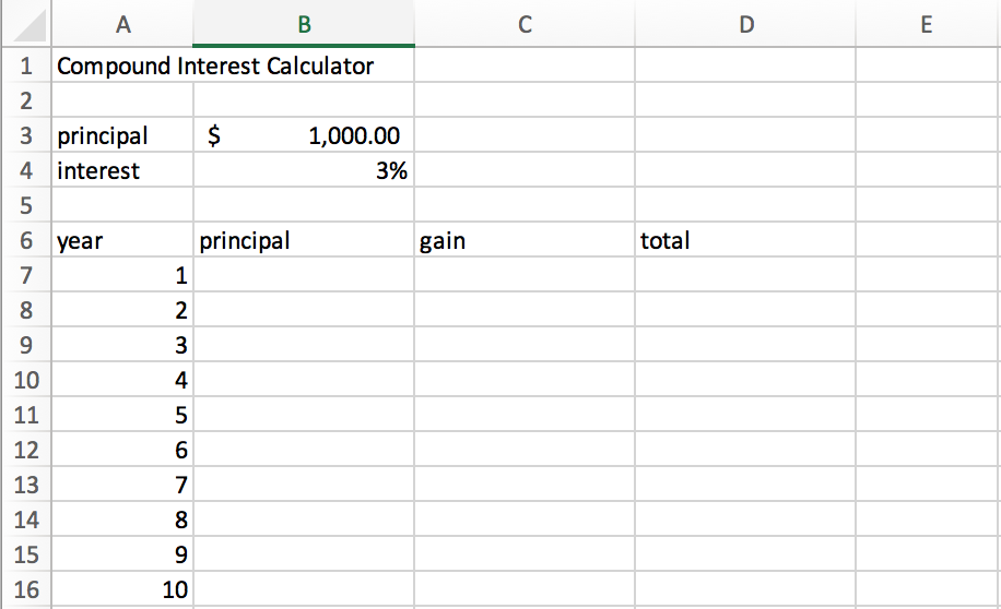
Let’s get started. Open up a blank excel spreadsheet and let’s make a template for our calculator. Start a few rows down with a column of “year” and input as many as you’d like, for mine I’m using 10 years. Beside “year” add columns for “principal”, “interest” and “total”. Next make labels for “principal” and “interest”, this is where you’ll be able to input your interest and principal that will affect the rest of the spreadsheet.

Great, we’ve got a template, now for the fun part. Input any principal and interest you’d like to use beside our “principal” and “interest” labels (cells B3 and B4). For my example, I’ll be using $1000 for principal and 3% for interest. In the “interest” cell (cell B4) make sure the cell is set to percentage otherwise you’ll need to input 0.03 instead of 3% for the calculation to work.
Time for our calculations. In the first row under our “principal” column (cell B7) we’re going to give it the value of our principal we’ve already made in B3. To do this simply click on the cell and type “=B3”.

For our “gain” column we’ll be multiplying our interest percentage by our principal to find the return on principal. We’ll also be adding a “$” to let excel know that this will be a repeating value. In the first row of the gain column (cell C7) type “=B7*B$4” to calculate the total gain on principal.

For our last column we’ll be summing the “principal” and “gain” columns to reach our yearly total. To do this type “=B7+C7”.

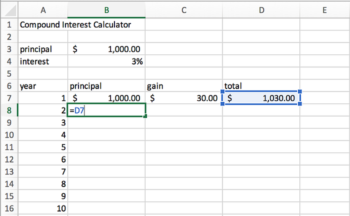
Lastly, we’ll be inputting one more row before letting excel work its magic. In the second row under principal (cell B8) we’re going to give it the value of our previous yearly total by typing “=D7”. This will let excel know that we’re starting each row from the total of the last row.
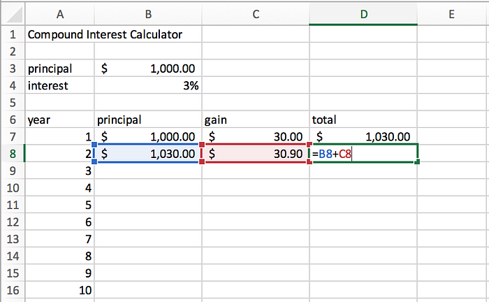
Input gain and total the same as we did for the last row only this time the “gain” column will be typed as “=B8*b$4” and the “total” column will be typed as “=B8+C8” because we are on row 8.
Now it’s time to leverage the power of Excel. We’ll be selecting the second row and extending it down the range of our years and Excel will fill in the table for us. The table wouldn’t fill without this second row because we need to include in our calculation that each row takes its principal from the last row’s total. To select our row simply click and drag the length of the 3 cells. A green box should be highlighted around the row now. Click and drag the corner of this box down to however many years you’d like Excel to fill.
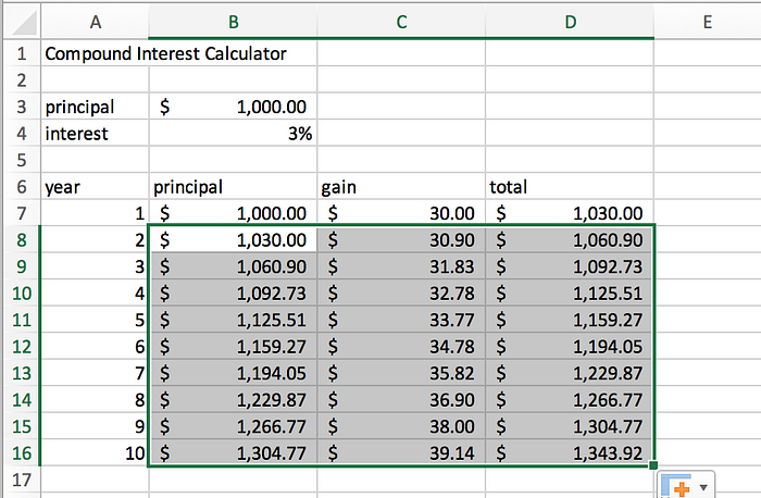
Congratulations! You’ve made your own compound calculator with Excel. You can change the values next to your principal and interest labels at any time and Excel will change the values in the entire table to match.
This spreadsheet style calculator is great to pick apart every detail of the compounding process as well as calculate any time interval you’d like with just a few tweaks to your rows.
